Introduction
“The nitrogen in our DNA, the calcium in our teeth, the iron in our blood, the carbon in our apple pies were made in the interiors of collapsing stars. We are made of starstuff.”
“If you wish to make an apple pie from scratch, you must first invent the universe.”
“We are like butterflies who flutter for a day and think it is forever.”
“The absence of evidence is not the evidence of absence.”
“We are star stuff which has taken its destiny into its own hands.”
Cosmos - Carl SaganThis post is the 4th and possibly, the last part of my introduction, to my latest cricket package yorkr. This is the 4th part of the introduction, the 3 earlier ones were
- Introducing cricket package yorkr-Part1:Beaten by sheer pace!.
- Introducing cricket package yorkr: Part 2-Trapped leg before wicket!
- Introducing cricket package yorkr: Part 3-Foxed by flight!
The 1st part included functions dealing with a specific match, the 2nd part dealt with functions between 2 opposing teams. The 3rd part dealt with functions between a team and all matches with all oppositions. This 4th part includes individual batting and bowling performances in ODI matches and deals with Class 4 functions.
If you are passionate about cricket, and love analyzing cricket performances, then check out my 2 racy books on cricket! In my books, I perform detailed yet compact analysis of performances of both batsmen, bowlers besides evaluating team & match performances in Tests , ODIs, T20s & IPL. You can buy my books on cricket from Amazon at $12.99 for the paperback and $4.99/$6.99 respectively for the kindle versions. The books can be accessed at Cricket analytics with cricketr and Beaten by sheer pace-Cricket analytics with yorkr A must read for any cricket lover! Check it out!!

d $4.99/Rs 320 and $6.99/Rs448 respectively
This post has also been published at RPubs yorkr-Part4 and can also be downloaded as a PDF document from yorkr-Part4.pdf.
You can clone/fork the code for the package yorkr from Github at yorkr-package
Checkout my interactive Shiny apps GooglyPlus (plots & tables) and Googly (only plots) which can be used to analyze IPL players, teams and matches.
Important note 1: Do check out all the posts on the python avatar of yorkr, namely ‘yorkpy’ in my post ‘Pitching yorkpy … short of good length to IPL – Part 1
Batsman functions
- batsmanRunsVsDeliveries
- batsmanFoursSixes
- batsmanDismissals
- batsmanRunsVsStrikeRate
- batsmanMovingAverage
- batsmanCumulativeAverageRuns
- batsmanCumulativeStrikeRate
- batsmanRunsAgainstOpposition
- batsmanRunsVenue
- batsmanRunsPredict
Bowler functions
- bowlerMeanEconomyRate
- bowlerMeanRunsConceded
- bowlerMovingAverage
- bowlerCumulativeAvgWickets
- bowlerCumulativeAvgEconRate
- bowlerWicketPlot
- bowlerWicketsAgainstOpposition
- bowlerWicketsVenue
- bowlerWktsPredict
Note: The yorkr package in its current avatar only supports ODI, T20 and IPL T20 matches.
library(yorkr)
library(gridExtra)
library(rpart.plot)
library(dplyr)
library(ggplot2)
rm(list=ls())
A. Batsman functions
1. Get Team Batting details
The function below gets the overall team batting details based on the RData file available in ODI matches. This is currently also available in Github at (https://github.com/tvganesh/yorkrData/tree/master/ODI/ODI-matches). However you may have to do this as future matches are added! The batting details of the team in each match is created and a huge data frame is created by rbinding the individual dataframes. This can be saved as a RData file
setwd("C:/software/cricket-package/york-test/yorkrData/ODI/ODI-matches")
india_details <- getTeamBattingDetails("India",dir=".", save=TRUE)
dim(india_details)
## [1] 11085 15sa_details <- getTeamBattingDetails("South Africa",dir=".",save=TRUE)
dim(sa_details)## [1] 6375 15nz_details <- getTeamBattingDetails("New Zealand",dir=".",save=TRUE)
dim(nz_details)## [1] 6262 15eng_details <- getTeamBattingDetails("England",dir=".",save=TRUE)
dim(eng_details)## [1] 9001 152. Get batsman details
This function is used to get the individual batting record for a the specified batsmen of the country as in the functions below. For analyzing the batting performances the following cricketers have been chosen
- Virat Kohli (Ind)
- M S Dhoni (Ind)
- AB De Villiers (SA)
- Q De Kock (SA)
- J Root (Eng)
- M J Guptill (NZ)
setwd("C:/software/cricket-package/york-test/yorkrData/ODI/ODI-matches")
kohli <- getBatsmanDetails(team="India",name="Kohli",dir=".")
## [1] "./India-BattingDetails.RData"dhoni <- getBatsmanDetails(team="India",name="Dhoni")## [1] "./India-BattingDetails.RData"devilliers <- getBatsmanDetails(team="South Africa",name="Villiers",dir=".")## [1] "./South Africa-BattingDetails.RData"deKock <- getBatsmanDetails(team="South Africa",name="Kock",dir=".")## [1] "./South Africa-BattingDetails.RData"root <- getBatsmanDetails(team="England",name="Root",dir=".")## [1] "./England-BattingDetails.RData"guptill <- getBatsmanDetails(team="New Zealand",name="Guptill",dir=".")## [1] "./New Zealand-BattingDetails.RData"3. Runs versus deliveries
Kohli, De Villiers and Guptill have a good cluster of points that head towards 150 runs at 150 deliveries.
p1 <-batsmanRunsVsDeliveries(kohli,"Kohli")
p2 <- batsmanRunsVsDeliveries(dhoni, "Dhoni")
p3 <- batsmanRunsVsDeliveries(devilliers,"De Villiers")
p4 <- batsmanRunsVsDeliveries(deKock,"Q de Kock")
p5 <- batsmanRunsVsDeliveries(root,"JE Root")
p6 <- batsmanRunsVsDeliveries(guptill,"MJ Guptill")
grid.arrange(p1,p2,p3,p4,p5,p6, ncol=3)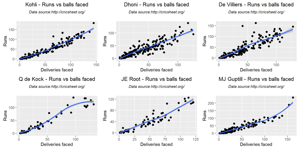
4. Batsman Total runs, Fours and Sixes
The plots below show the total runs, fours and sixes by the batsmen
kohli46 <- select(kohli,batsman,ballsPlayed,fours,sixes,runs)
p1 <- batsmanFoursSixes(kohli46,"Kohli")
dhoni46 <- select(dhoni,batsman,ballsPlayed,fours,sixes,runs)
p2 <- batsmanFoursSixes(dhoni46,"Dhoni")
devilliers46 <- select(devilliers,batsman,ballsPlayed,fours,sixes,runs)
p3 <- batsmanFoursSixes(devilliers46, "De Villiers")
deKock46 <- select(deKock,batsman,ballsPlayed,fours,sixes,runs)
p4 <- batsmanFoursSixes(deKock46,"Q de Kock")
root46 <- select(root,batsman,ballsPlayed,fours,sixes,runs)
p5 <- batsmanFoursSixes(root46,"JE Root")
guptill46 <- select(guptill,batsman,ballsPlayed,fours,sixes,runs)
p6 <- batsmanFoursSixes(guptill46,"MJ Guptill")
grid.arrange(p1,p2,p3,p4,p5,p6, ncol=3)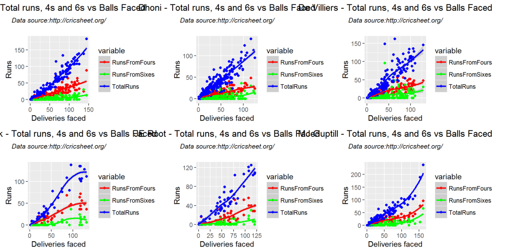
5. Batsman dismissals
The type of dismissal for each batsman is shown below
p1 <-batsmanDismissals(kohli,"Kohli")
p2 <- batsmanDismissals(dhoni, "Dhoni")
p3 <- batsmanDismissals(devilliers, "De Villiers")
p4 <- batsmanDismissals(deKock,"Q de Kock")
p5 <- batsmanDismissals(root,"JE Root")
p6 <- batsmanDismissals(guptill,"MJ Guptill")
grid.arrange(p1,p2,p3,p4,p5,p6, ncol=3)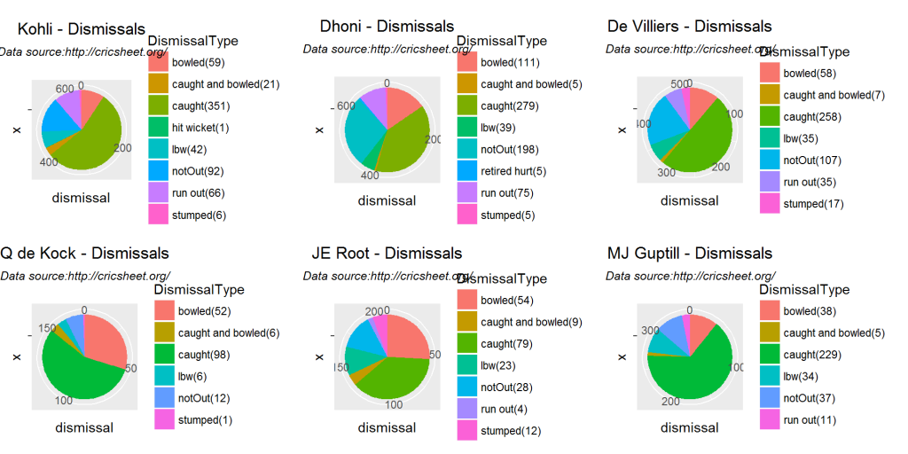
6. Runs versus Strike Rate
De villiers has the best strike rate among all as there are more points to the right side of the plot for the same runs. Kohli and Dhoni do well too. Q De Kock and Joe Root also have a very good spread of points though they have fewer innings.
p1 <-batsmanRunsVsStrikeRate(kohli,"Kohli")
p2 <- batsmanRunsVsStrikeRate(dhoni, "Dhoni")
p3 <- batsmanRunsVsStrikeRate(devilliers, "De Villiers")
p4 <- batsmanRunsVsStrikeRate(deKock,"Q de Kock")
p5 <- batsmanRunsVsStrikeRate(root,"JE Root")
p6 <- batsmanRunsVsStrikeRate(guptill,"MJ Guptill")
grid.arrange(p1,p2,p3,p4,p5,p6, ncol=3)
7. Batsman moving average
Kohli’s average is on a gentle increase from below 50 to around 60’s. Joe Root performance is impressive with his moving average of late tending towards the 70’s. Q De Kock seemed to have a slump around 2015 but his performance is on the increase. Devilliers consistently averages around 50. Dhoni also has been having a stable run in the last several years.
p1 <-batsmanMovingAverage(kohli,"Kohli")
p2 <- batsmanMovingAverage(dhoni, "Dhoni")
p3 <- batsmanMovingAverage(devilliers, "De Villiers")
p4 <- batsmanMovingAverage(deKock,"Q de Kock")
p5 <- batsmanMovingAverage(root,"JE Root")
p6 <- batsmanMovingAverage(guptill,"MJ Guptill")
grid.arrange(p1,p2,p3,p4,p5,p6, ncol=3)
8. Batsman cumulative average
The functions below provide the cumulative average of runs scored. As can be seen Kohli and Devilliers have a cumulative runs rate that averages around 48-50. Q De Kock seems to have had a rocky career with several highs and lows as the cumulative average oscillates between 45-40. Root steadily improves to a cumulative average of around 42-43 from his 50th innings
p1 <-batsmanCumulativeAverageRuns(kohli,"Kohli")
p2 <- batsmanCumulativeAverageRuns(dhoni, "Dhoni")
p3 <- batsmanCumulativeAverageRuns(devilliers, "De Villiers")
p4 <- batsmanCumulativeAverageRuns(deKock,"Q de Kock")
p5 <- batsmanCumulativeAverageRuns(root,"JE Root")
p6 <- batsmanCumulativeAverageRuns(guptill,"MJ Guptill")
grid.arrange(p1,p2,p3,p4,p5,p6, ncol=3)
9. Cumulative Average Strike Rate
The plots below show the cumulative average strike rate of the batsmen. Dhoni and Devilliers have the best cumulative average strike rate of 90%. The rest average around 80% strike rate. Guptill shows a slump towards the latter part of his career.
p1 <-batsmanCumulativeStrikeRate(kohli,"Kohli")
p2 <- batsmanCumulativeStrikeRate(dhoni, "Dhoni")
p3 <- batsmanCumulativeStrikeRate(devilliers, "De Villiers")
p4 <- batsmanCumulativeStrikeRate(deKock,"Q de Kock")
p5 <- batsmanCumulativeStrikeRate(root,"JE Root")
p6 <- batsmanCumulativeStrikeRate(guptill,"MJ Guptill")
grid.arrange(p1,p2,p3,p4,p5,p6, ncol=3)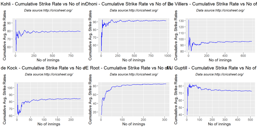
10. Batsman runs against opposition
Kohli’s best performances are against Australia, West Indies and Sri Lanka
batsmanRunsAgainstOpposition(kohli,"Kohli")
batsmanRunsAgainstOpposition(dhoni, "Dhoni")
Kohli’s best performances are against Australia, Pakistan and West Indies
batsmanRunsAgainstOpposition(devilliers, "De Villiers")
Quentin de Kock average almost 100 runs against India and 75 runs against England
batsmanRunsAgainstOpposition(deKock, "Q de Kock")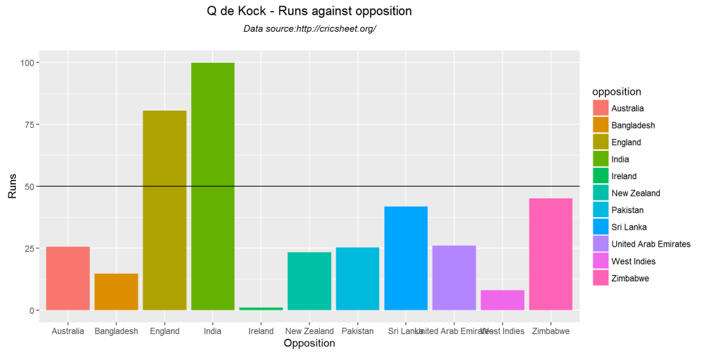
Root’s best performances are against South Africa, Sri Lanka and West Indies
batsmanRunsAgainstOpposition(root, "JE Root")
batsmanRunsAgainstOpposition(guptill, "MJ Guptill")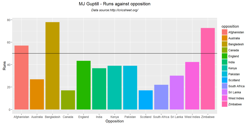
11. Runs at different venues
The plots below give the performances of the batsmen at different grounds.
batsmanRunsVenue(kohli,"Kohli")
batsmanRunsVenue(dhoni, "Dhoni")
batsmanRunsVenue(devilliers, "De Villiers")
batsmanRunsVenue(deKock, "Q de Kock")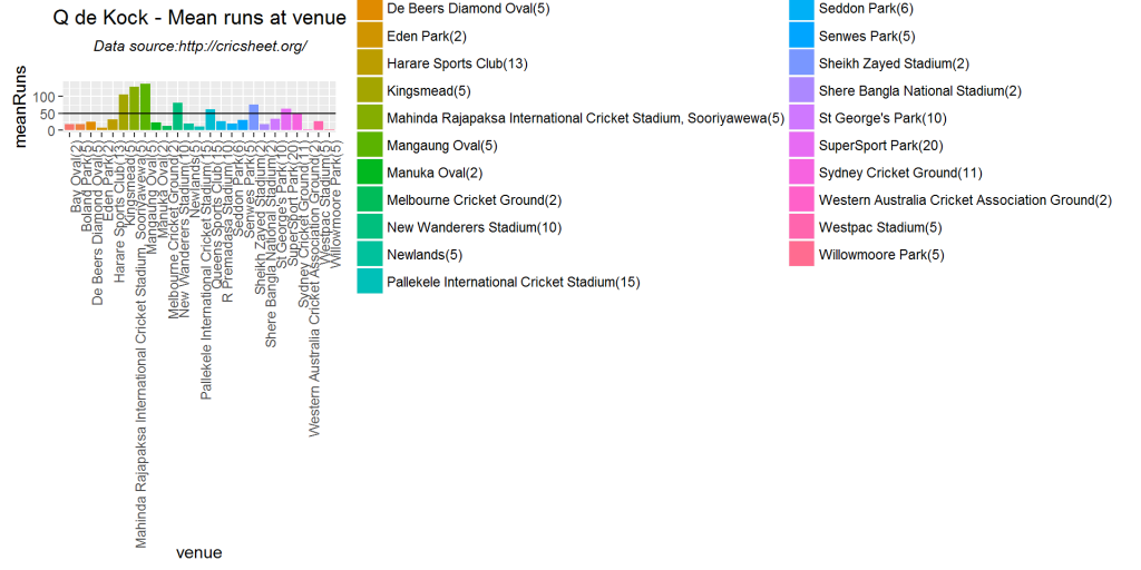
batsmanRunsVenue(root, "JE Root")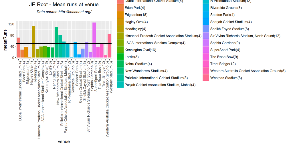
batsmanRunsVenue(guptill, "MJ Guptill")
12. Predict number of runs to deliveries
The plots below use rpart classification tree to predict the number of deliveries required to score the runs in the leaf node. For e.g. Kohli takes 66 deliveries to score 64 runs and for higher number of deliveries scores around 115 runs. Devilliers needs
par(mfrow=c(1,3))
par(mar=c(4,4,2,2))
batsmanRunsPredict(kohli,"Kohli")
batsmanRunsPredict(dhoni, "Dhoni")
batsmanRunsPredict(devilliers, "De Villiers")
par(mfrow=c(1,3))
par(mar=c(4,4,2,2))
batsmanRunsPredict(deKock,"Q de Kock")
batsmanRunsPredict(root,"JE Root")
batsmanRunsPredict(guptill,"MJ Guptill")
B. Bowler functions
13. Get bowling details
The function below gets the overall team bowling details based on the RData file available in ODI matches. This is currently also available in Github at (https://github.com/tvganesh/yorkrData/tree/master/ODI/ODI-matches). The bowling details of the team in each match is created and a huge data frame is created by rbinding the individual dataframes. This can be saved as a RData file
setwd("C:/software/cricket-package/york-test/yorkrData/ODI/ODI-matches")
ind_bowling <- getTeamBowlingDetails("India",dir=".",save=TRUE)
dim(ind_bowling)
## [1] 7816 12aus_bowling <- getTeamBowlingDetails("Australia",dir=".",save=TRUE)
dim(aus_bowling)## [1] 9191 12ban_bowling <- getTeamBowlingDetails("Bangladesh",dir=".",save=TRUE)
dim(ban_bowling)## [1] 5665 12sa_bowling <- getTeamBowlingDetails("South Africa",dir=".",save=TRUE)
dim(sa_bowling)## [1] 3806 12sl_bowling <- getTeamBowlingDetails("Sri Lanka",dir=".",save=TRUE)
dim(sl_bowling)## [1] 3964 1214. Get bowling details of the individual bowlers
This function is used to get the individual bowling record for a specified bowler of the country as in the functions below. For analyzing the bowling performances the following cricketers have been chosen
- R A Jadeja (Ind)
- Ravichander Ashwin (Ind)
- Mitchell Starc (Aus)
- Shakib Al Hasan (Ban)
- Ajantha Mendis (SL)
- Dale Steyn (SA)
jadeja <- getBowlerWicketDetails(team="India",name="Jadeja",dir=".")
ashwin <- getBowlerWicketDetails(team="India",name="Ashwin",dir=".")
starc <-  getBowlerWicketDetails(team="Australia",name="Starc",dir=".")
shakib <-  getBowlerWicketDetails(team="Bangladesh",name="Shakib",dir=".")
mendis <-  getBowlerWicketDetails(team="Sri Lanka",name="Mendis",dir=".")
steyn <-  getBowlerWicketDetails(team="South Africa",name="Steyn",dir=".")
15. Bowler Mean Economy Rate
Shakib Al Hassan is expensive in the 1st 3 overs after which he is very economical with a economy rate of 3-4. Starc, Steyn average around a ER of 4.0
p1<-bowlerMeanEconomyRate(jadeja,"RA Jadeja")
p2<-bowlerMeanEconomyRate(ashwin, "R Ashwin")
p3<-bowlerMeanEconomyRate(starc, "MA Starc")
p4<-bowlerMeanEconomyRate(shakib, "Shakib Al Hasan")
p5<-bowlerMeanEconomyRate(mendis, "A Mendis")
p6<-bowlerMeanEconomyRate(steyn, "D Steyn")
grid.arrange(p1,p2,p3,p4,p5,p6, ncol=3)
16. Bowler Mean Runs conceded
Ashwin is expensive around 6 & 7 overs
p1<-bowlerMeanRunsConceded(jadeja,"RA Jadeja")
p2<-bowlerMeanRunsConceded(ashwin, "R Ashwin")
p3<-bowlerMeanRunsConceded(starc, "M A Starc")
p4<-bowlerMeanRunsConceded(shakib, "Shakib Al Hasan")
p5<-bowlerMeanRunsConceded(mendis, "A Mendis")
p6<-bowlerMeanRunsConceded(steyn, "D Steyn")
grid.arrange(p1,p2,p3,p4,p5,p6, ncol=3)
17. Bowler Moving average
RA jadeja and Mendis’ performance has dipped considerably, while Ashwin and Shakib have improving performances. Starc average around 4 wickets
p1<-bowlerMovingAverage(jadeja,"RA Jadeja")
p2<-bowlerMovingAverage(ashwin, "Ashwin")
p3<-bowlerMovingAverage(starc, "M A Starc")
p4<-bowlerMovingAverage(shakib, "Shakib Al Hasan")
p5<-bowlerMovingAverage(mendis, "Ajantha Mendis")
p6<-bowlerMovingAverage(steyn, "Dale Steyn")
grid.arrange(p1,p2,p3,p4,p5,p6, ncol=3)
17. Bowler cumulative average wickets
Starc is clearly the most consistent performer with 3 wickets on an average over his career, while Jadeja averages around 2.0. Ashwin seems to have dropped from 2.4-2.0 wickets, while Mendis drops from high 3.5 to 2.2 wickets. The fractional wickets only show a tendency to take another wicket.
p1<-bowlerCumulativeAvgWickets(jadeja,"RA Jadeja")
p2<-bowlerCumulativeAvgWickets(ashwin, "Ashwin")
p3<-bowlerCumulativeAvgWickets(starc, "M A Starc")
p4<-bowlerCumulativeAvgWickets(shakib, "Shakib Al Hasan")
p5<-bowlerCumulativeAvgWickets(mendis, "Ajantha Mendis")
p6<-bowlerCumulativeAvgWickets(steyn, "Dale Steyn")
grid.arrange(p1,p2,p3,p4,p5,p6, ncol=3)
18. Bowler cumulative Economy Rate (ER)
The plots below are interesting. All of the bowlers seem to average around 4.5 runs/over. RA Jadeja’s ER improves and heads to 4.5, Mendis is seen to getting more expensive as his career progresses. From a ER of 3.0 he increases towards 4.5
p1<-bowlerCumulativeAvgEconRate(jadeja,"RA Jadeja")
p2<-bowlerCumulativeAvgEconRate(ashwin, "Ashwin")
p3<-bowlerCumulativeAvgEconRate(starc, "M A Starc")
p4<-bowlerCumulativeAvgEconRate(shakib, "Shakib Al Hasan")
p5<-bowlerCumulativeAvgEconRate(mendis, "Ajantha Mendis")
p6<-bowlerCumulativeAvgEconRate(steyn, "Dale Steyn")
grid.arrange(p1,p2,p3,p4,p5,p6, ncol=3)
19. Bowler wicket plot
The plot below gives the average wickets versus number of overs
p1<-bowlerWicketPlot(jadeja,"RA Jadeja")
p2<-bowlerWicketPlot(ashwin, "Ashwin")
p3<-bowlerWicketPlot(starc, "M A Starc")
p4<-bowlerWicketPlot(shakib, "Shakib Al Hasan")
p5<-bowlerWicketPlot(mendis, "Ajantha Mendis")
p6<-bowlerWicketPlot(steyn, "Dale Steyn")
grid.arrange(p1,p2,p3,p4,p5,p6, ncol=3)
20. Bowler wicket against opposition
#Jadeja's' best pertformance are against England, Pakistan and West Indies
bowlerWicketsAgainstOpposition(jadeja,"RA Jadeja")
#Ashwin's bets pertformance are against England, Pakistan and South Africa
bowlerWicketsAgainstOpposition(ashwin, "Ashwin")
#Starc has good performances against India, New Zealand, Pakistan, West Indies
bowlerWicketsAgainstOpposition(starc, "M A Starc")
bowlerWicketsAgainstOpposition(shakib,"Shakib Al Hasan")
bowlerWicketsAgainstOpposition(mendis, "Ajantha Mendis")
#Steyn has good performances against India, Sri Lanka, Pakistan, West Indies
bowlerWicketsAgainstOpposition(steyn, "Dale Steyn")
21. Bowler wicket at cricket grounds
bowlerWicketsVenue(jadeja,"RA Jadeja")
bowlerWicketsVenue(ashwin, "Ashwin")
bowlerWicketsVenue(starc, "M A Starc")## Warning: Removed 2 rows containing missing values (geom_bar).
bowlerWicketsVenue(shakib,"Shakib Al Hasan")
bowlerWicketsVenue(mendis, "Ajantha Mendis")
bowlerWicketsVenue(steyn, "Dale Steyn")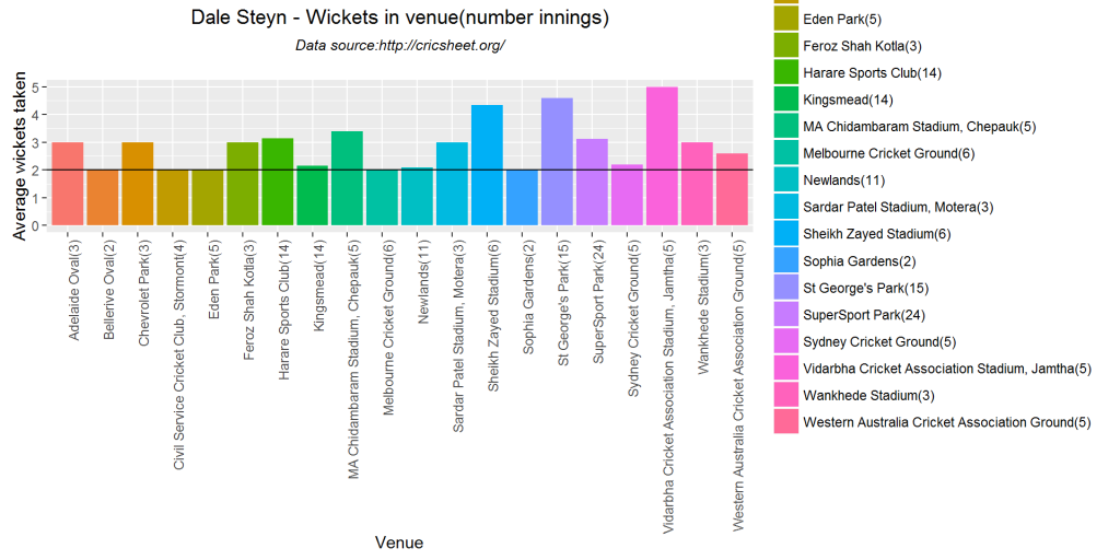
22. Get Delivery wickets for bowlers
Thsi function creates a dataframe of deliveries and the wickets taken
setwd("C:/software/cricket-package/york-test/yorkrData/ODI/ODI-matches")
jadeja1 <- getDeliveryWickets(team="India",dir=".",name="Jadeja",save=FALSE)
ashwin1 <- getDeliveryWickets(team="India",dir=".",name="Ashwin",save=FALSE)
starc1 <- getDeliveryWickets(team="Australia",dir=".",name="MA Starc",save=FALSE)
shakib1 <- getDeliveryWickets(team="Bangladesh",dir=".",name="Shakib",save=FALSE)
mendis1 <- getDeliveryWickets(team="Sri Lanka",dir=".",name="Mendis",save=FALSE)
steyn1 <- getDeliveryWickets(team="South Africa",dir=".",name="Steyn",save=FALSE)
23. Predict number of deliveries to wickets
#Jadeja and Ashwin need around 22 to 28 deliveries to make a break through
par(mfrow=c(1,2))
par(mar=c(4,4,2,2))
bowlerWktsPredict(jadeja1,"RA Jadeja")
bowlerWktsPredict(ashwin1,"RAshwin")
#Starc and Shakib provide an early breakthrough producing a wicket in around 16 balls. Starc's 2nd wicket comed around the 30th delivery
par(mfrow=c(1,2))
par(mar=c(4,4,2,2))
bowlerWktsPredict(starc1,"MA Starc")
bowlerWktsPredict(shakib1,"Shakib Al Hasan")
#Steyn and Mendis take 20 deliveries to get their 1st wicket
par(mfrow=c(1,2))
par(mar=c(4,4,2,2))
bowlerWktsPredict(mendis1,"A Mendis")
bowlerWktsPredict(steyn1,"DSteyn")
Conclusion
This concludes the 4 part introduction to my new R cricket package yorkr for ODIs. I will be enhancing the package to handle Twenty20 and IPL matches soon. You can fork/clone the code from Github at yorkr.
The yaml data from Cricsheet have already beeen converted into R consumable dataframes. The converted data can be downloaded from Github at yorkrData. There are 3 folders – ODI matches, ODI matches between 2 teams (oppnAllMatches), ODI matches between a team and the rest of the world (all matches,all oppositions).
As I have already mentioned I have around 67 functions for analysis, however I am certain that the data has a lot more secrets waiting to be tapped. So please do go ahead and run any machine learning or statistical learning algorithms on them. If you do come up with interesting insights, I would appreciate if attribute the source to Cricsheet(http://cricsheet.org), and my package yorkr and my blog Giga thoughts*, besides dropping me a note.
Hope you have a great time with my yorkr package!
Important note: Do check out my other posts using yorkr at yorkr-posts
Also see
- Introducing cricketr! : An R package to analyze performances of cricketers
- Cricket analytics with cricketr in paperback and Kindle versions
- My TEDx talk on the “Internet of Things”
- Bend it like Bluemix,MongoDB with autoscaling – Part 1
- The mind of a programmer
- Fun simulation of a chain in Android
- Taking cricketr for a spin-Part 1
- Latency,throughput implications for the cloud
- Hand detection through haar-training: A hands-on approach
- Cricket analytics with cricketr


9 thoughts on “Introducing cricket package yorkr:Part 4-In the block hole!”