Neural Networks: The mechanics of backpropagation

The initial work in the ‘Backpropagation Algorithm’ started in the 1980’s and led to an explosion of interest in Neural Networks and the application of backpropagation

The ‘Backpropagation’ algorithm computes the minimum of an error function with respect to the weights in the Neural Network. It uses the method of gradient descent. The combination of weights in a multi-layered neural network, which minimizes the error/cost function is considered to be a solution of the learning problem.

In the Neural Network above
$out_{o1} =\sum_{i} w_{i}*x_{i}$
$E = 1/2(target - out)^{2}$
$\partial E/\partial out= 1/2*2*(target - out) *-1 = -(target - out)$
$\partial E/\partial w_{i} =\partial E/\partial y* \partial y/\partial w_{i}$
$\partial E/\partial w_{i} = -(target - out) * x_{i}$

Checkout my book ‘Deep Learning from first principles: Second Edition – In vectorized Python, R and Octave’. My book starts with the implementation of a simple 2-layer Neural Network and works its way to a generic L-Layer Deep Learning Network, with all the bells and whistles. The derivations have been discussed in detail. The code has been extensively commented and included in its entirety in the Appendix sections. My book is available on Amazon as paperback ($18.99) and in kindle version($9.99/Rs449).

Perceptrons and single layered neural networks can only classify, if the sample space is linearly separable. For non-linear decision boundaries, a multi layered neural network with backpropagation is required to generate more complex boundaries.The backpropagation algorithm, computes the minimum of the error function in weight space using the method of gradient descent. This computation of the gradient, requires the activation function to be both differentiable and continuous. Hence the sigmoid or logistic function is typically chosen as the activation function at every layer.

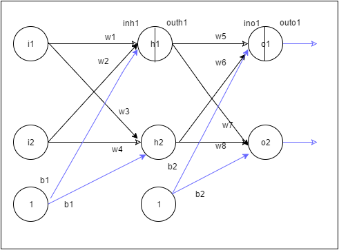
This post looks at a 3 layer neural network with 1 input, 1 hidden and 1 output. To a large extent this post is based on Matt Mazur’s detailed “A step by step backpropagation example“, and Prof Hinton’s “Neural Networks for Machine Learning” at Coursera and a few other sources.

While Matt Mazur’s post uses example values, I generate the formulas for the gradient derivatives for each weight in the hidden and input layers. I intend to implement a vector version of backpropagation in Octave, R and Python. So this post is a prequel to that.

The 3 layer neural network is as below

Some basic derivations which are used in backpropagation

Chain rule of differentiation
Let y=f(u)
and u=g(x) then
$\partial y/\partial x = \partial y/\partial u * \partial u/\partial x$

An important result
$y=1/(1+e^{-z})$
Let $x= 1 + e^{-z}$ then
$y = 1/x$
$\partial y/\partial x = -1/x^{2}$
$\partial x/\partial z = -e^{-z}$

Using the chain rule of differentiation we get
$\partial y/\partial z = \partial y/\partial x * \partial x/\partial z$
$=-1/(1+e^{-z})^{2}* -e^{-z} = e^{-z}/(1+e^{-z})^{2}$
Therefore $\partial y/\partial z = y(1-y)$ -(A)

1) Feed forward network
The net output at the 1st hidden layer
$in_{h1} = w_{1}i_{1} + w_{2}i_{2} + b_{1}$
$in_{h2} = w_{3}i_{1} + w_{4}i_{2} + b_{1}$

The sigmoid/logistic function function is used to generate the activation outputs for each hidden layer. The sigmoid is chosen because it is continuous and also has a continuous derivative

$out_{h1} = 1/1+e^{-in_{h1}}$
$out_{h2} = 1/1+e^{-in_{h2}}$

The net output at the output layer
$in_{o1} = w_{5}out_{h_{1}} + w_{6}out_{h_{2}} + b_{2}$
$in_{o2} = w_{7}out_{h_{1}} + w_{8}out_{h_{2}} + b_{2}$

Total error
$E_{total} = 1/2\sum (target - output)^{2}$
$E_{total} = E_{o1} + E_{o2}$
$E_{total} = 1/2(target_{o_{1}} - out_{o_{1}})^{2} + 1/2(target_{o_{2}} - out_{o_{2}})^{2}$

2)The backwards pass
In the backward pass we need to compute how the squared error changes with changing weight. i.e we compute $\partial E_{total}/\partial w_{i}$ for each weight $w_{i}$ . This is shown below

A squared error is assumed

Error gradient with $w_{5}$

$\partial E_{total}/\partial w_{5} = \partial E_{total}/\partial out_{o_{1}} * \partial out_{o_{1}}/\partial in_{o_{1}} * \partial in_{o_{1}}/ \partial w_{5}$ -(B)

Since
$E_{total} = 1/2\sum (target - output)^{2}$
$E_{total} = 1/2(target_{o_{1}} - out_{o_{1}})^{2} + 1/2(target_{o_{2}} - out_{o_{2}})^{2}$
$\partial E _{total}/\partial out_{o1} = \partial E_{o1}/\partial out_{o1} + \partial E_{o2}/\partial out_{o1}$
$\partial E _{total}/\partial out_{o1} = \partial /\partial _{out_{o1}}[1/2(target_{01}-out_{01})^{2}- 1/2(target_{02}-out_{02})^{2}]$
$\partial E _{total}/\partial out_{o1} = 2 * 1/2*(target_{01} - out_{01}) *-1 + 0$

Now considering the 2nd term in (B)
$\partial out_{o1}/\partial in_{o1} = \partial/\partial in_{o1} [1/(1+e^{-in_{o1}})]$

Using result (A)
$\partial out_{o1}/\partial in_{o1} = \partial/\partial in_{o1} [1/(1+e^{-in_{o1}})] = out_{o1}(1-out_{o1})$

The 3rd term in (B)
$\partial in_{o1}/\partial w_{5} = \partial/\partial w_{5} [w_{5}*out_{h1} + w_{6}*out_{h2}] = out_{h1}$
$\partial E_{total}/\partial w_{5}=-(target_{o1} - out_{o1}) * out_{o1} *(1-out_{o1}) * out_{h1}$

Having computed $\partial E_{total}/\partial w_{5}$ , we now perform gradient descent, by computing a new weight, assuming a learning rate $\alpha$
$w_{5}^{+} = w_{5} - \alpha * \partial E_{total}/\partial w_{5}$

If we do this for $\partial E_{total}/\partial w_{6}$ we would get
$\partial E_{total}/\partial w_{6}=-(target_{02} - out_{02}) * out_{02} *(1-out_{02}) * out_{h2}$

3)Hidden layer

We now compute how the total error changes for a change in weight $w_{1}$
$\partial E_{total}/\partial w_{1}= \partial E_{total}/\partial out_{h1}* \partial out_{h1}/\partial in_{h1} * \partial in_{h1}/\partial w_{1}$ – (C)

Using
$E_{total} = E_{o1} + E_{o2}$ we get
$\partial E_{total}/\partial w_{1}= (\partial E_{o1}/\partial out_{h1}+ \partial E_{o2}/\partial out_{h1}) * \partial out_{h1}/\partial in_{h1} * \partial in_{h1}/\partial w_{1}$
$\partial E_{total}/\partial w_{1}=(\partial E_{o1}/\partial out_{h1}+ \partial E_{o2}/\partial out_{h1}) * out_{h1}*(1-out_{h1})*i_{1}$ -(D)

Considering the 1st term in (C)
$\partial E_{total}/\partial out_{h1}= \partial E_{o1}/\partial out_{h1}+ \partial E_{o2}/\partial out_{h1}$

Now
$\partial E_{o1}/\partial out_{h1} = \partial E_{o1}/\partial out_{o1} *\partial out_{o1}/\partial in_{01} * \partial in_{o1}/\partial out_{h1}$
$\partial E_{o2}/\partial out_{h1} = \partial E_{o2}/\partial out_{o2} *\partial out_{o2}/\partial in_{02} * \partial in_{o2}/\partial out_{h1}$

which gives the following
$\partial E_{o1}/\partial out_{o1} *\partial out_{o1}/\partial in_{o1} * \partial in_{o1}/\partial out_{h1} =-(target_{o1}-out_{o1}) *out_{o1}(1-out_{o1})*w_{5}$ – (E)
$\partial E_{o2}/\partial out_{o2} *\partial out_{o2}/\partial in_{02} * \partial in_{o2}/\partial out_{h1} =-(target_{o2}-out_{o2}) *out_{o2}(1-out_{o2})*w_{6}$ – (F)

Combining (D), (E) & (F) we get
$\partial E_{total}/\partial w_{1} = -[(target_{o1}-out_{o1}) *out_{o1}(1-out_{o1})*w_{5} + (target_{o2}-out_{o2}) *out_{o2}(1-out_{o2})*w_{6}]*out_{h1}*(1-out_{h1})*i_{1}$

This can be represented as
$\partial E_{total}/\partial w_{1} = -\sum_{i}[(target_{oi}-out_{oi}) *out_{oi}(1-out_{oi})*w_{j}]*out_{h1}*(1-out_{h1})*i_{1}$

With this derivative a new value of $w_{1}$ is computed
$w_{1}^{+} = w_{1} - \alpha * \partial E_{total}/\partial w_{1}$

Hence there are 2 important results
At the output layer we have
a) $\partial E_{total}/\partial w_{j}=-(target_{oi} - out_{oi}) * out_{oi} *(1-out_{oi}) * out_{hi}$
At each hidden layer we compute
b) $\partial E_{total}/\partial w_{k} = -\sum_{i}[(target_{oi}-out_{oi}) *out_{oi}(1-out_{oi})*w_{j}]*out_{hk}*(1-out_{hk})*i_{k}$

Backpropagation, was very successful in the early years, but the algorithm does have its problems for e.g the issue of the ‘vanishing’ and ‘exploding’ gradient. Yet it is a very key development in Neural Networks, and the issues with the backprop gradients have been addressed through techniques such as the momentum method and adaptive learning rate etc.

In this post. I derive the weights at the output layer and the hidden layer. As I already mentioned above, I intend to implement a vector version of the backpropagation algorithm in Octave, R and Python in the days to come.

Watch this space! I’ll be back

P.S. If you find any typos/errors, do let me know!

References
1. Neural Networks for Machine Learning by Prof Geoffrey Hinton
2. A Step by Step Backpropagation Example by Matt Mazur
3. The Backpropagation algorithm by R Rojas
4. Backpropagation Learning Artificial Neural Networks David S Touretzky
5. Artificial Intelligence, Prof Sudeshna Sarkar, NPTEL

Also see my other posts
1. Introducing QCSimulator: A 5-qubit quantum computing simulator in R
2. Design Principles of Scalable, Distributed Systems
3. A method for optimal bandwidth usage by auctioning available bandwidth using the OpenFlow protocol
4. De-blurring revisited with Wiener filter using OpenCV
5. GooglyPlus: yorkr analyzes IPL players, teams, matches with plots and tables
6. Re-introducing cricketr! : An R package to analyze performances of cricketers

To see all my posts go to ‘Index of Posts‘