Introduction: After my initial encounter with IBM’s Quantum Experience, and my playing around with qubits, quantum gates and trying out the Bell experiment I can now say that I am fairly hooked to quantum computing.
So, I decided that before going any further, that I needed to spend a little time more, getting to know more about the basics of Dirac’s bra-ket notation, qubits and ensuring that my knowledge is properly “chunked” ( See Learning to Learn: Powerful mental tools to master tough subjects, a really good course!!)
So, I started to look around for material on Quantum Computing, and finally landed on the classic course “Quantum Mechanics and Quantum Computing”, from University of California, Berkeley by Prof Umesh V Vazirani at edX. I have started to audit the course (listen in, without doing the assignments). The Prof is unbelievably good, and makes the topic both interesting and absorbing. This post is based on my notes of week 1 & 2 lectures. I have tried to articulate as best as I can, what I have understood of the lectures, though I would strongly recommend you to, at least audit the archived course. By the way, I also had to refresh my knowledge of basic trigonometry and linear algebra. My knowledge of the basics of matrix manipulation, vectors etc. were buried deep within the sands of time. Luckily for me, they were reasonably intact.
A) Quantum states
A hydrogen atom has 1 electron in orbit. The electron can be either in the idle state or in the excited state. We can represent the idle state with |0> and the excited state with |1>, which is Dirac’s ‘ket’ notation.

This electron will be in a superposition state which is represented by
Ψ = α |0> + β |1> where α & β are complex numbers and obey | α|2 + | β|2 = 1
For e.g. we could have the superposition state
It can be seen that | α|2 = 
For a complex number α = a+ bi == > | α| =


B) Measurement
However, when the electron or the qubit is measured, the state of superposition collapses to either |0> or |1> with the following probability’s
The resulting state is
|0> with probability | α|2
|1> with probability | β |2
And | α|2 + | β|2 = 1 because the sum of the probabilities must add up to 1 i.e.

C) Geometric interpretation
Let us consider a qubit that is in a superposition state
Ψ = α |0> + β |1> where α & β are complex numbers and obey | α|2 + | β|2 = 1
We can write this as a vector 
It can be seen that if


and


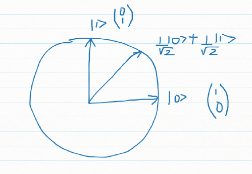


Measuring a qubit in standard basis
If we represent the qubit geometrically then the superposition can be represented as a vector which makes an angle 

Measuring this 
The output is is |0> with probability 
|1> with probability

D) Measuring a qubit in any basis

The qubit can be measured in any arbitrary basis. For e.g. if
Ψ = α |0> + β |1> and we have the diagonal basis
|u>| and |u’> as shown and Ψ makes an angle 
|u> with probability cos2Θ
And |u’> with probability sin2Θ
E) K Qubit system
Let us assume that we have a Quantum System with k qubits
|0>, |1>, |2>… |k-1>
The qubit will be in a superimposed state
Ψ = α0 |0>+ α1 |1> + α2|2> + … + αk-1 |k-1>
Where αj is a complex vector with the property ∑ αj = 1
Here Ψ is a unit vector in a K dimensional complex vector space, known as Hilbert Space
For e.g. a 3 qubit quantum system
Then P(0) = ½ P(1) = ¼ and P(2) = ¼ ∑Pj = 1

We could also write
Or
Ψ = α0 |0>+ α1 |1> + α2|2> + … + αk-1 |k-1>

F) Measuring the angle between 2 complex vectors
To measure the angle between 2 complex vectors
And
we need to take the inner product of the complex conjugate of the 1st vector and the 2nd
cosΘ = inner product =>


For e.g.
If 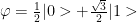
And

Then the angle between these 2 vectors are obtained by taking the inner product
cosΘ = ½ * 1/√2 + √3/2 * ½
G) Measuring Ψ in |+> or |-> basis
For e.g. if
Then we can specify/measure Ψ in |+> or |-> basis as follow
|+> = 1/√2(|0> + |1>) and |-> = 1/√2(|0> – |1>)
Or |0> = 1/√2(|+> + |->) and |1> = 1/√2(|+> – |->)
We can write
Ψ= α|+> + β|->
Substituting for |0> and |1> in (A) we get

H) Quantum gates
I) Clifford gates
Pauli gates
a) Pauli X
The Pauli X gate does a bit flip
|0> ==> X|0> ==> |1>
|1> ==> X|1> ==> |0>
and is represented

b) Pauli Z
This gates does a phase flip and is represented as the 2 x 2 unitary matrix

c) Pauli Y
The Pauli operator Y does both a bit and a phase flip. The Y operator is represented as

K) Superposition gates
Superposition is the concept that adding quantum states together results in a new quantum state. There are 3 gates that perform superposition of qubits the H, S and S’ gate.
a) H gate (Hadamard gate)
The H gate, also known as the Hadamard Gate when applied |0> state results in the qubit being half the time in |0> and the other half in |1>
The H gate can be represented as
1/√2

b) S gate
The S gate can be represented as

c) S’ gate
And the S’ gate is

L) Non-Clifford Gates
The quantum gates discussed in my earlier post Pauli X, Y, Z, H, S and S1 are members of a special group of gates known as the ‘Clifford group’.
The non-Clifford gates, discussed are the T and Tǂ gates
These are given by
T =
Tǂ =


M) 2 qubit system
A 2 qubit system
A 2 qubit system is a superposition of all possible 2 qubit states. A 2 qubit system and can be represented as
Ψ = α00 |00> + α01 |01> + α10 |10> + α11 |11>
Measuring the 2 qubit system, as earlier, results in the collapse of the superposition and the result is one of 4 qubit states. The probability of the measure state is the square of the amplitude | αij|2
N) Entanglement
A 2 qubit system in which we have
Ψ = α0 |0> + α1 |1> and Φ= β0 |0> + β1 |1> the superimposed state is obtained by taking the tensor product of the 2 qubits
Where 

The state
Ψ = 1/√2|00> + 1/√2|11>
Is called an ‘entangled’ state because it cannot be reduced to a product of 2 vectors
N) 2 qubit gates

A 2 qubit system is a superposition of all possible 2 qubit states. A 2 qubit system and can be represented as
Ψ = α00 |00> + α01 |01> + α10 |10> + α11 |11>
Measuring the 2 qubit system, as earlier, results in the collapse of the superposition and the result is one of 4 qubit states. The probability of the measure state is the square of the amplitude | αij|2
More specifically a 2 qubit system in which we have
Ψ = α0 |0> + α1 |1> and Φ= β0 |0> + β1 |1> the superimposed state is obtained by taking the tensor product of the 2 qubits
Where 
The state
Ψ = 1/√2|00> + 1/√2|11>
Is called an ‘entangled’ state because it cannot be reduced to a product of 2 vectors
A quantum gate is a 2 x 2 unitary matrix U such that
α0 |0> + α1 |1> == > Quantum Gate == > β0|0> + β1 |1>
Unitary functions: In mathematics, a complex square matrix U is unitary if its conjugate transpose U* is also its inverse
If
U=
And U* =
Then
UU* = I where I is the Identity matrix


2 qubit gates is 4 x 4 unitary matrix
For a 2 qubit that is in the superposition state
Ψ = α00 |00> + α01 |01> + α10 |10> + α11 |11>
A 2 qubit gate’s operation on Ψ is


One important 2 qubit gate is the CNOT gate which is shown below
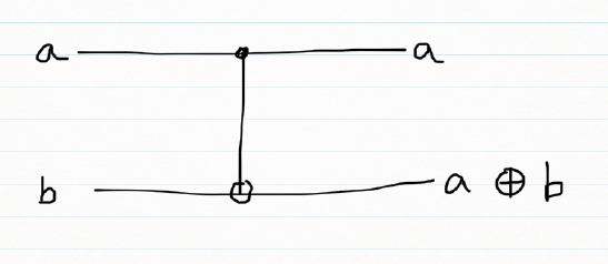
The CNOT gate is represented by the following unitary matrix

If 2 2×2 qubit gates were applied to 2 qubits the composite gate would be Tensor product of the 2 matrices
u1 =
u2 =
then
U=
U =
The above product is also known as the Kronecker product


O) Tensor product of 2 qubits
Ψ = α0 |0> + α1 |1> and Φ= β0 |0> + β1 |1>
$latex \varphi \otimes \phi= α0 β0|0>|0> + α0 β1|0>|1> + α1 β0|1>|0> + α1 β1|1>|1>
= α0 β0|00> + α0 β1|01> + α1 β0|10> + α1 β1|11>

If a Z gate and a Hadamard gate H were applied on 2 qubits, it is interest to know what the resulting composite gate would be.
Z = 
The composite gate is obtained by the tensor product of
Hence the result of the composite gate is
=
=


which is the entangled state.
Conclusion: This post includes most of the required basics to get started on Quantum Computing. I will probably add another post detailing the operations of the Quantum Gates on qubits.
Note:
1.The equations and matrices have been created using LaTeX notation using the online LaTex equation creator
2. The figures have been created using the app Bamboo Paper, which I think is cooler than creating in Powerpoint
Also see
1.Venturing into IBM’s Quantum Experience
2. Going deeper into IBM’s Quantum Experience!
You may also like
1. Sixer – R package cricketr’s new Shiny avatar
2. Natural language processing: What would Shakespeare say?
3. Sea shells on the seashore
4. How to program – Some essential tips
5. Rock N’ Roll with Bluemix, Cloudant & NodeExpress
6. The Many Faces of Latency


Yes, Vazirani’s course on edx is really good. For beginners I would suggest another very good set of lectures by Micheal Nielsen, they are available on Youtube (titled Quantum Computing for the Determined).
LikeLike